Everyday One Step Forward

Introduction

---

The entropy coding is another very important part of video coding. The purpose of entorpy coding is to compress the syntax data, residual pixel data. The h264 standard specifies two types of entropy coding: Context-based Adaptive Binary Arithmetic Coding (CABAC) and Variable-Length Coding (VLC)

Variable Length Coding (VLC)

---

• Exp-Golomb Entropy Coding:

Exp-Golomb codes are variable lenght codes with regular construction. The codeword is constructed as:

\([M zeros][1][INFO]\)

INFO is an M-bits field carrying information. Each Exp-Golomb codeword can be constructed by the encoder based on its index code_num:

\(INFO = code\_num + 1 - 2^M\)

A codeword can be decoded as followed step:

1. Read in M leading zeros followed by 1
2. Read M-bit INFO field
3. \(code\_num = 2^M + INFO -1\)

The is a table for 1-exp-golomb codewords:

code_num	codewrod
0	1
1	010
2	011
3	00100
4	00101
5	00110
6	00111
7	0001000
8	0001001

• Unsigned Direct Mapping:

Flaged as ue(v), code_num = v. Used for MB type, reference frame index and others

• Signed Mapping:

Flaged as se(v), used for motion vector difference, delta QP and others. v is mapped to code_num as follows:

\(code\_num = 2|v| (v<0)\)

\(code\_num = 2|v|-1 (v \geq 0)\)

• Mapped Symbols:

Flaged as me(v). Parameter v is mapped to code_num according to a table sepcified in the standard spec. The mapping is used or CBP.

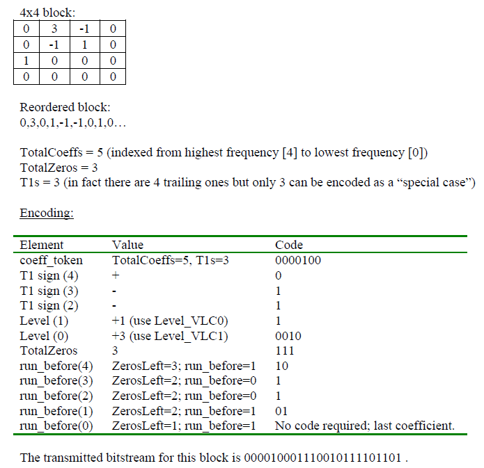
• Context-based Adaptive Variable Length Coding (CAVLC):

The CAVLC is used to encode residual, zig-zag ordered 4x4(and 2x2) blocks of transform coefficients. The CAVLC encoding proceeds as follows:

1. Encode the number of coefficients and trailing ones (coeff_token)
2. Encode the sign of each T1
3. Encode the levels of the remaining non-zero coefficients
4. Encode the total number of zeros before the last coefficient
5. Encode each run of zeros

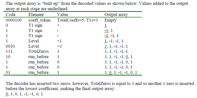
At decoder part, do the reverse operation:

Context-based Adaptive Binary Arithmetic Coding (CABAC)

---

Here is an artical introduce the CABAC algorithm in H264.

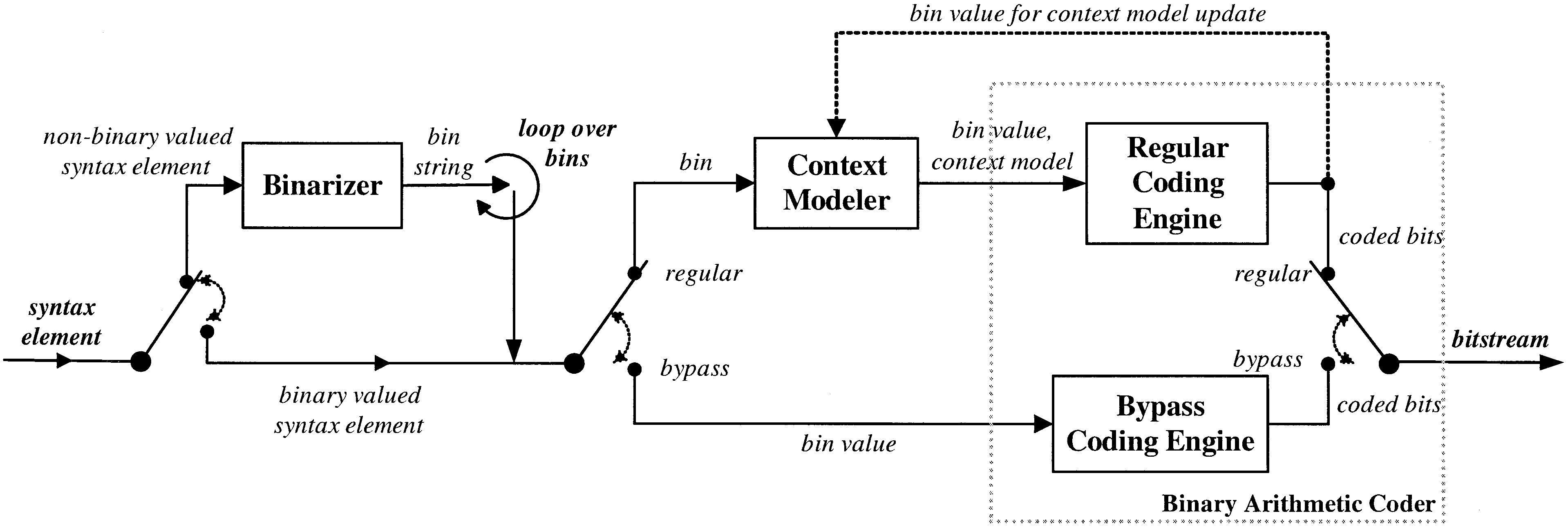
• The CABAC Framework:

The CABAC encoding process consist of, at most, three steps:

1. binarization
2. context modeling
3. binary arithmetic coding

• Binarization:

There several types of binarization method:

1. unary and truncated unary binarization
2. kth order Exp-Golomb binarization
3. fixed length binarization

In the binarization step, a given nonbinary valued syntax element is uniquely mapped to a binary sequence, a so-called bin string. When a binary valued syntax element is given, this initial step is bypassed.

• Context Modeling:

In the so-called regular coding mode, prior to the actual arithmetic coding process the given binary decision which, in the sequel, we will refer to as a bin, enters the context modeling stage, where a probability model is selected such that the corresponding choice may depend on previously encoded syntax elements or bins. Then, after the assignment of a context model the bin value along with its associated model is passed to the regular coding engine, where the final stage of arithmetic encoding together with a subsequent model updating takes place.

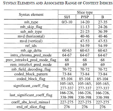
Each syntax element has context indices and each context indices has an corresponding status. The status will be used to calculate the current context's probability. Furthermore, the status will be updated after being used to encoding one bin. Then the next time the bin of the context will use the updated syntax for encoding.

H264's spec provided the table for syntax elements and associated range of context indices:

• Binary Arithmetic Coding:

Binary arithmetic coding is based on the principle of recursive interval subdivision that involves the following elementary multiplication operation. Suppose the lease probable symbol (LPS) is \(p_{LPS} \in (0,0.5]\). The given interval is represented by lower bound \(L\) and its width(range) \(R\). Then the given interval is subdivided into two subintervals, \(R_{LPS} = R \centerdot p_{LPS}\) which is associated with the \(LPS\), and the \(R_{MPS} = R - R_{LPS}\) assigned to most probable symbol (MPS), which have the probability \(1-p_{LPS}\)

The cost of multiplication is big, thus CABAC proposed a method with multiplication free, which is table search based method. The basic idea of multiplication free approach is to project both the legal range \([R_{min}, R_{max})\) of interval width R and the probability range associated with the \(LPS\) onto a small set of representive value \(Q = \{Q_0,...,Q_{K-1}\}\) and \(P = \{p_0,...,p_{N-1}\}\) respectively. The realization of H264 choose \(k=4\) and \(N=64\), then the values of \(R \centerdot P_{LPS}\) are obtained by a \(K \times N (4 \times 64)\) table

ps. One special operation is bypass coding mode, which be used for nearly uniform distributed \((p \approx 0.5)\)

• Probability Estimation:

The basic idea of the new multiplication free binary arithmetic coding scheme for H.264/AVC relies on the assumption that the estimated probabilities of each context model can be represented by a sufficiently limited set of representative values. For H264 CABAC, 64 representative probabilities values

\(p_{\sigma} = \alpha \centerdot p_{\sigma - 1}\) for all \(\sigma = 1,...,63\)

\(\alpha = (\frac{0.01875}{0.5})^{1/63}\) and \(p_0 = 0.5\)

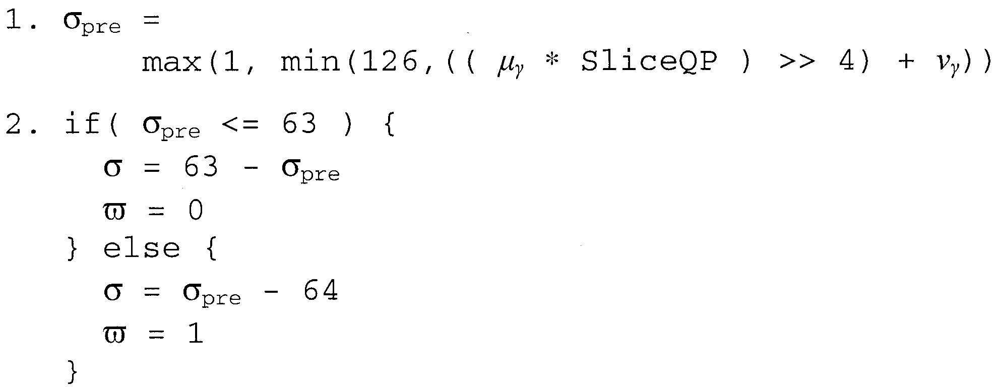
Each context model in CABAC can be completely determined by two parameters: its current estimate of the \(LPS\) probability, which is characterized by index \(\sigma\) between 1 and 63, and its value of MPS \(\varpi\) being either 0 or 1. Thus, probability estimation in CABAC is performed by using a total number of 128 different probability states, each of them efficiently represented by a 7-bit integer value. In fact, one of the state indices \((\sigma = 63)\) is related to an autonomous, nonadaptive state with a fixed value of MPS, which is only used for encoding of binary decisions before termination of the arithmetic codeword, as further explained below. Therefore, only 126 probability states are effectively used for the representation and adaptation of all (adaptive) context models.

• Probability Update:

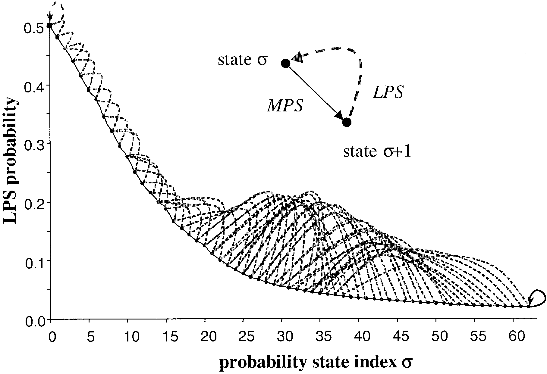
As already stated above, all probability models in CABAC with one exception are (backward) adaptive models, where an update of the probability estimation is performed after each symbol has been encoded. Actually, for a given probability state, the update depends on the state index and the value of the encoded symbol identified either as a LPS or a MPS. As a result of the updating process, a new probability state is derived, which consists of a potentially modified LPS probability estimate and, if necessary, a modified MPS value.

If \(\sigma = 62\) is the following value is also MPS \(\varpi\), then \(\sigma\) keep equal to 62 until a LPS come.

if \(\sigma = 0\) LPS reach equal probability status. \(\sigma\) keep equal to 0 but the value of LPS and MPS will switch, which means the previous LPS's probability increased to become MPS, then if the next time comes still LPS, \(\sigma = \sigma + 1\) will not stick to \(\sigma = 0\)

• Initialization and Reset of Probability States:

CABAC provides a built-in mechanism for incorporating some a priori knowledge about the source statistics in the form of appropriate initialization values for each of the probability models. This so-called initialization process for context models allows an adjustment of the initial probability states in CABAC on two levels.

• Regular Coding Mode:

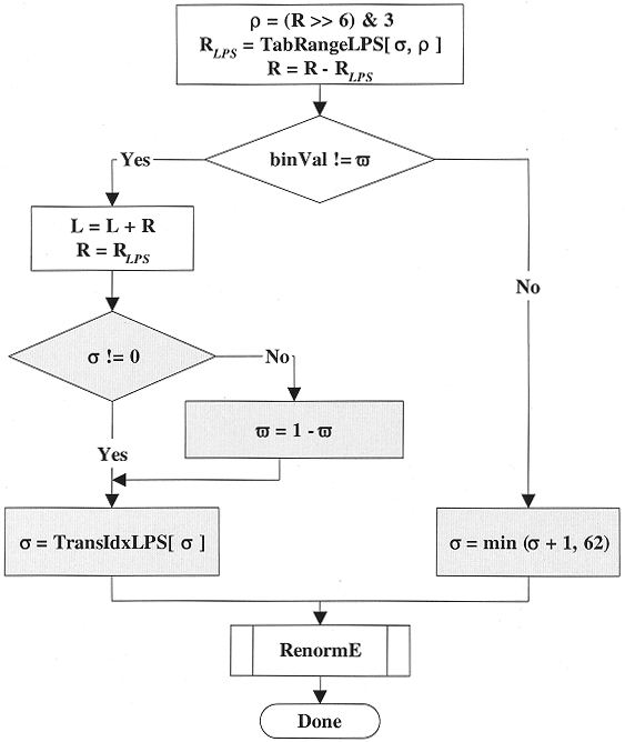
In the first and major step, the current interval is subdivided according to the given probability estimates. The current interval range \(R\) is approximated by a quantized value \(Q(R)\) using an equi-partition of the whole range \(2^8 \leq R < 2^9\) [256, 512) into four cells. But instead of using the corresponding representative quantized range values \(Q_0, Q_1, Q_2, Q_3\) explicitly in the CABAC engine, \(Q(R)\) is only addressed by its quantizer index \(\rho\), which is

\(\rho = (R>>6) \& 3\)

Then, this index \(\rho\) and the probability state \(\sigma\) index are used as entries in a 2-D table TabRangeLPS to determine the (approximate) LPS related subinterval range. Here, the table TabRangeLPS contains all 64 4 pre-computed product values \(p_{\sigma} \centerdot Q_{\rho}\) for \(0 \leq \sigma \leq 63\) and \(0 \leq \rho \leq 3\) in 8-bit precision.

\(R_{LPS} = TabRangeLPS(\sigma, \rho)\)

• Bypass Coding Mode:

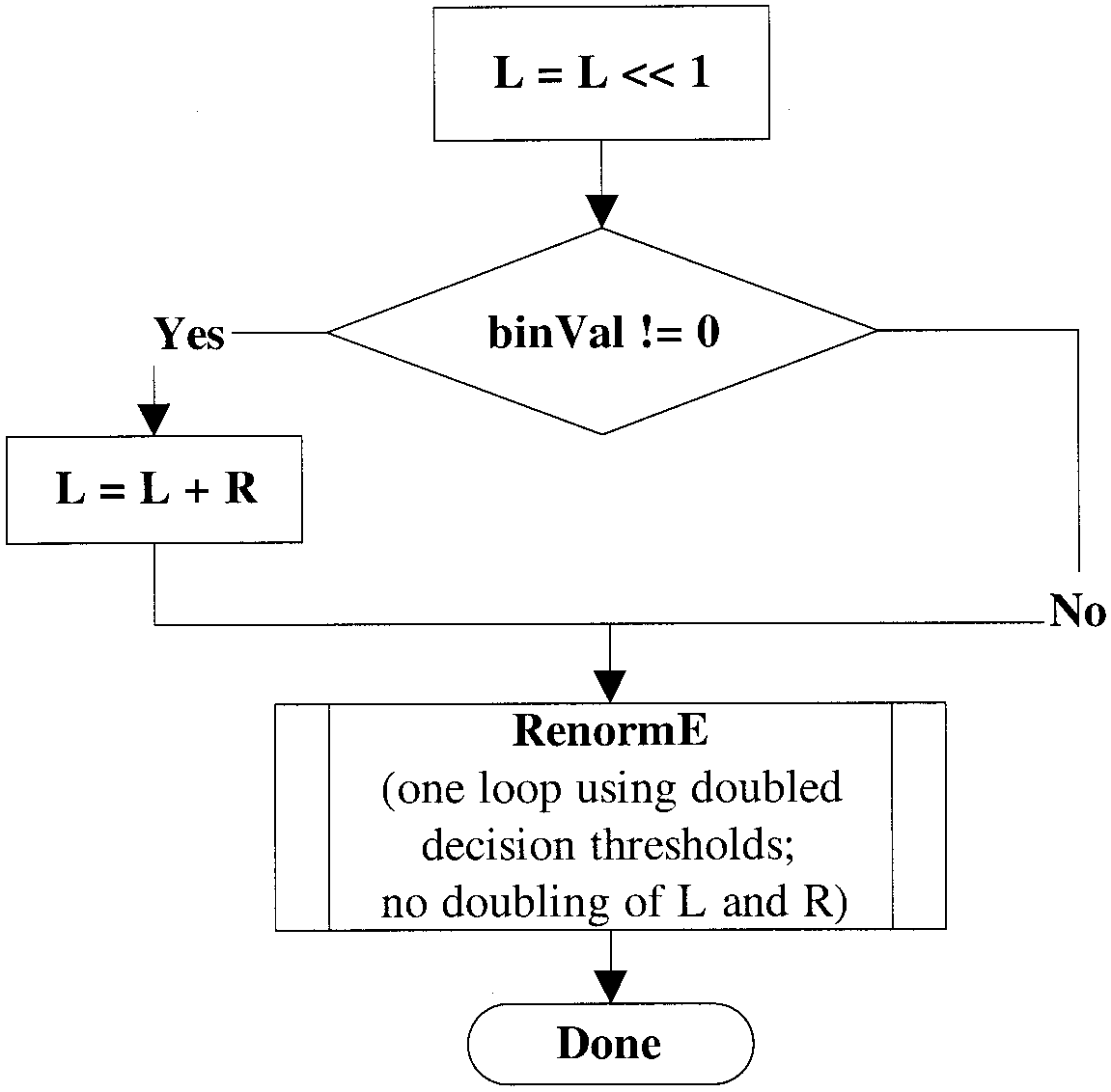
To speed up the encoding (and decoding) of symbols, for which \(R-R_{LPS} \approx R_{LPS} \approx R/2\) is assumed to hold, the regular arithmetic encoding process as described in the previous paragraph is simplified to a large extent. First, a “bypass” of the probability estimation and update process is established, and second, the interval subdivision is performed such that two equisized subintervals are provided in the interval subdivision stage. But instead of explicitly halving the current interval range R, the variable L is doubled before choosing the lower or upper subinterval depending on the value of the symbol to encode (0 or 1, respectively). In this way, doubling of L and R in the subsequent renormalization is no longer required provided that the renormalization in the bypass is operated with doubled decision thresholds.

• Renormalization and Carry-Over Control:

A renormalization operation after interval subdivision is required whenever the new interval range R no longer stays within its legal range of \([2^8, 2^9)\) . Each time renormalization must be carried out, one or more bits can be output. However, in certain cases, the polarity of the output bits will be resolved in subsequent output steps, i.e., carry propagation might occur in the arithmetic encoder.

• Termination of Arithmetic Code Word:

A special fixed, i.e., nonadapting probability state with index \(\sigma = 63\) was designed such that the associated table entries \(TabRangeLPS[63, \rho]\), and hence \(R_{LPS}\) are determined by a fixed value of 2 regardless of the given quantized range index \(\rho\). This guarantees that for the terminating syntax element in a slice which, in general, is given by the LPS value of the end of slice flag, 7 bits of output are produced in the related renormalization step. Two more disambiguating bits are needed to terminate the arithmetic codeword for a given slice. By preventing the decoder from performing a renormalization after recovering the terminating syntax element, the decoder never reads more bits than were actually produced by the encoder for that given slice.